Installing R and R packages locally

This week I learned how to install R and R packages in a local home directory while working on a server.  I made a quick step-by-step tutorial and placed it on GitHub to keep as a reminder for myself.  It was much easier than I thought it would be. Hopefully others will find it useful too!

cowplot: arrange ggplot2 figures in a grid

Sadly, cowplot doesn't create plots of cows, but it would be fun if it did! So I thought the next best thing would be to include some cow data. :p

What is cowplot? cowplot is a fun little R package that labels and arranges figures created by ggplot2 into a grid. It also has a nice publication-ready theme for ggplot2 plots. I started using cowplot a few weeks ago and thought I would write a short blog post on the handy features.

For the last few years if I wanted to arrange plots created by ggplot2 into a grid, I would use either the multiplot() function from the Cookbook for R or the arrange_ggplot2() function from Stephen Turner's blog Getting Genetics Done. If I were creating these plots for a publication, I would also want to add labels (e.g. A, B, C, etc) to the arranged plots to be able to refer to individual plots. I would also typically fiddle with the default theme in ggplot2 to remove the default gray background and grid lines (personal preference thing).

Why is it useful? cowplot offers two really cool features:

1. The default theme in cowplot has no gray background and no grid lines. It is very similar to ggplot2's theme_classic(), but the main difference is mostly related to the font sizes.
2. There are two functions plot_grid() and ggdraw() that allow the user to arrange and label figures in grid. The plots can be arranged according to a specified number of columns (or rows), horizontally (or vertically), and can be labeled. 

For this blogpost, I found a data set that measures the butterfat content from 100 cows of different breeds and different ages. Very appropriate! :) The data set is located in the PAWSR R package. 

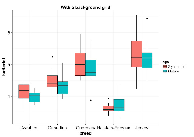
Here used ggplot2 to create box plots comparing the butterfat content of the different breeds along the x-axis and colored by the age of the cows.  The first set of box plots uses the default cowplot theme. The second uses ggplot2's classic theme and the default theme. To get ggplot2's classic theme and default theme in cowplot, use classic_theme() and theme_gray(), respectively.  Notice how the default theme in cowplot does not contain the gray background and gridlines.  Also, the color of the axis ticks are black instead of gray the ggplot2 default gray theme. 

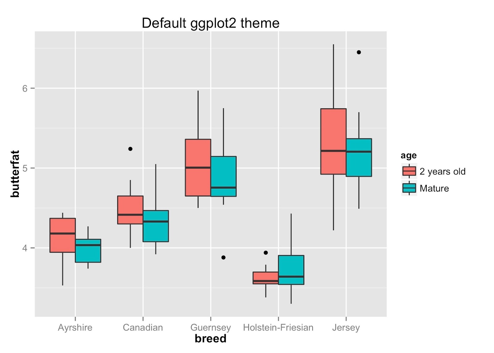
Density plots of the butter fat content colored by age and faceted by breed.

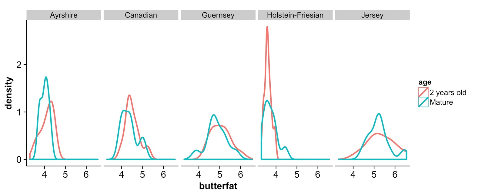
Now, sometimes there is a reason to  have the grid lines loaded. In that case, you can use the background_grid() function.

The second thing I really like about cowplot is the built in functions to arrange and label figures in a grid. There are two ways of doing this.  The simplest way is to use plot_grid() which takes in a list of ggplot2 plot names and arranges them in a grid according to the specified number of columns (or rows) and how to arrange the plots (vertically or horizontally), etc.  You can also provide a set of labels (and label sizes).

Because figure D is more wide than the other three figures, we may want to manually create the grid of plots to be able to specify the width and height of each figure individually.  In that case, you want to use the ggdraw() function with the draw_plot() function.  The ggdraw() function is the base layer and then you can place individual plots at arbitrary locations using the draw_plot() function.

As a final note, you can also check out the functions draw_label(), draw_line(), and  draw_text() which allow you to draw lines and text on top of the individual plots.

Backed my first Kickstarter: Reader

Today I backed my first Kickstarter which will create Reader: Dragging Science Publications into the 21st Century.  As someone who reads a lot of science publications, I think this is a fantastic idea! Reader is a viewer that will render manuscripts in a web browser (phone, tablet and computer) to allow the reader to interact and discuss papers, bookmark papers & citations, load figures and inline context of the paper (no software or app to install).  

It's always a hassle to flip back and forth between the results section, figures, figure legend, and references when reading a paper in the traditional format. Now all of that will be changed with Reader. Here is an demo of a publication from their website. I look forward to start using Reader in August 2015 (expected date of completion).  

Angel food cake with chocolate whipped cream

Happy Fourth of July! One of my favorite summer desserts (and one of my favorite Fourth of July desserts) is angel food cake with whipped cream and fresh fruit.  In the hot days of summer, there is something particularly nice about this cake.  It's light, fluffy and just sweet enough to balance out the whipped cream and fruit.  Technically, I'm cheating by starting with a box cake mix (very rare for me), but the boxed cake mix is pretty good in this case!

Ingredients:
- 14oz heavy cream
- 1 box angel food cake mix
- strawberries, diced
- blueberries

Optional:
- 1/4 cup granulated sugar
- 2 tbsp cocco powder

Recipe:

1) Mix box cake mix and 1 1/4 cups water on high for 1 min. Start the blender slowly and then move faster to avoid cake mix flying everywhere.  Place cake mix in an angel food cake bundt pan.

2) Bake angel food cake at 350 degrees for 32-35 mins (until golden brown). Be careful to not under bake the cake mix.

Let the cake cool completely.

3) Whip the heavy cream for 1min on high. Slowly add granulated sugar and coco powder.  Continue to whip the cream until stiff peaks have formed. Be careful to not over mix (or you'll end up with butter!).

My favorite way to serve the cake is simply with a dollop of chocolate whipped cream and fresh fruit.

Happy 4th of July everyone!

Tutorial on mapping WGBS data using Bismark

I recently created a tutorial for the Harvard edX PH525.8x Case Study on DNA Methylation Analysis. This tutorial is a step-by-step guide of starting with raw Whole Genome Bisulfite Sequencing (WGBS) reads (SRA or fastq files), apply quality control filters, mapping mapping the filtered reads using Bismark and extracting the methylation calls for downstream analyses such as importing the methylation calls in R to find differently methylated CpGs or differentially methylated regions (see the bsseq R/Bioconductor package for more information).

As an example, we extracted six paired tumor-normal WGBS samples from Ziller et al. (2013) (PMID: 23925113). We have provided the coverage files (only chromosome 22) produced by Bismark in the colonCancerWGBS Github repository for others to use as a data example in R.

I hope others find the tutorial useful for the analysis of their own data!

Influential works in Data-Driven Discovery

A recent initiative to fund data-driven discoveries was completed last year by the Gordon and Betty Moore Foundation. Over 1,100 applications were received and each application had the opportunity to cite five "influential works in the general field of 'Big Data' for scientific discovery".  An analysis was done to see which works were cited the most and in what genres these works were from.  A paper summarizing the results was posted on arXiv on March 30, 2015 and had some interesting results that I wanted to share!

First, I was happy to see I have read several of the most cited influential works, but this also gave me a nice summer reading list of things I haven't read (I think this will basically be my #tbt (throwback Thursday) data-science papers for the next year)!  It was such a great list of works that I wanted to share the most cited influential works on here (each cited at least 10 times):

1. MapReduce [Dean and Ghemawat, 2008] - 63 (citations)
2. Fourth Paradigm [Hey et al., 2009] - 51
3. Elements of Statistical Learning [Hastie et al., 2009] - 43
4. Initial sequencing of the human genome [Lander et al., 2001] - 30
5. A mathematical theory of communication [Shannon, 2001] - 24
6. Sloan Digital Sky Survey [York et al., 2000] - 23
7. BLAST [Altschu et al., 1990] - 20
8. Lasso [Tibshirani et al., 1996] - 19
9. Latent Dirichlet allocation [Blei et al., 2003] - 19
10. EM algorithm [Demster et al., 1977] - 17
11. Support vector networks [Cortes and Vapnik, 1995] - 17
12. Random forest [Breiman, 2001] - 15
13. Pattern Recognition [Bishop et al., 2006] - 14
14. Anatomy of web search engine [Brin and Page, 1998] - 14
15. Numerical Recipes [Press, 2007] - 13
16. Boostrap methods [Efron, 1979] - 11
17. Equation of state calculations [Metropolis et al., 1953] - 11
18. Exploratory data analysis [Tukey, 1977] - 11
19. Probability reasoning [Pearl, 1988] - 11
20. PageRank [Page et al., 1999] - 10
21. Bayesian Data Analysis [Gelman et al., 2013] - 10
22. Unreasonable effectiveness of data [Halevy et al., 2009] - 10

Other cool things about this article:

• The R programming language and the IPython Notebook programming environment were highlighted. The authors state the "R language is one of the leading programming languages, and was referenced a significant number of times".  Similarly, the IPython Notebook "is noteworthy as one of the few open source software toolkits for both programming and data analysis that is not database, algorithm or programming language". 
• Classic/foundational ideas such as Bayes Theorem, Metropolis-Hastings Algorithm, lasso, bootstrap, Expectation-Maximization (EM) Algorithm were sprinkled throughout the article. These ideas are almost standard in any statistics curriculum and are incredibly powerful and useful tools when analyzing data. 
• The concepts of 'exploratory data analysis' (EDA) and 'data visualization' got a major shout out with Tukey's and Tufte's essential works.  These concepts are critical in the analysis of data and are often overlooked or treated as assumed knowledge.  I would argue that these concepts should be included as a major portion of any course based around teaching the concepts of data analysis.  

So, how many have of these have you read??

Pasta alla Carbonara

Pasta alla carbonara is one of those wonderfully decadent recipes that is an easy dinner during the week or perfect for a special date night! One of my good friends from Sicily recently showed me how to make pasta all carbonara the traditional Italian way which does not have cream, wine or stock (which was a big surprise to me since that's the typical way it is made in the US). Once you try this recipe, you won't even miss the cream! 

Ingredients: 

- 1 package of bacon

- 1 box of pasta (campanelle, farfella, penne, spaghetti, etc)

- 4 fresh eggs

- 1/2 cup parmesan cheese

- salt, pepper

Optional: chopped parsley

Recipe: 

1) Bring a pot of salted water to boil and cook pasta to al dente according to the directions (subtract 1-2 minutes from directions).  

2) At the same time that the water is boiling, chop raw bacon into bite size pieces. In a large pan, sauté bacon until golden brown. 

3) Using a slotted spoon, take the bacon off the pan and on to a plate with a towel to drain some of the fat.  At this point, you can turn off the heat and pour some of the rendered bacon fat out of the pan (but I prefer to keep all the bacon fat).  It just adds extra flavor! :)

4) By this point the pasta should be just finished cooking at perfect al dente and the pan with the rendered bacon fat should be off the heat. In the same pan with the rendered bacon fat, add the pasta, bacon and 4 eggs.  Make sure you mix everything as you add the eggs to prevent any scrambled eggs. The heat from the pasta will slightly cook the eggs. Add the parmesan cheese. Top with salt & pepper.

This recipe cooks so fast and is delicious. Seriously. You won't be disappointed! :)