Sampling Points Proportional to Intensity in an Image

A few months ago Aaron Lun shared some code with me to sample points based on intensity of pixels in an image. With his permission, I thought it would be fun to share it here!

The idea is you start with some image (either in a JPEG or PNG format). Here I'm using Rafa's twitter profile picture in a JPEG format.

I'm using the readJPEG() function from the R jpeg package to read in the JPEG image. Alternatively, you can use the readPNG() function from the R png package to read in a PNG image. If you read the help file of readJPEG(), it says it "reads an image from a JPEG file/content into a raster array". OK, first off what do we mean by raster? You can think of a raster image as a rectangular grid of pixels. In the help file for the readJPEG() function, it states "most common files decompress into RGB channels (3 channels)" where RGB stands for red, green and blue.

So, this means for each pixel in the original image, we should expect 3 values (one for red, green and blue). These values range between 0 and 1 and can be thought of the intensity of each color in the image. Below, I'm showing the intensity values from the three channels colored on the same scale (top row) and colored in the red, green and blue scales (bottom row).

To get the intensity of how light a particular pixel is, we can just average the values across the three channels. Next, we flip the intensity scale by subtracting the intensity scale from 1 to see how dark/black a particular pixel is. This makes the previously dark areas now light and vice versa (top left figure below). To control the contrast of intensity, you can just take powers of the intensity values. The lighter the background, the better the contrast will be between the individual and background on the original scale. Depending on the background in the original image, the skin tone, etc you may need to tinker with the contrast. I've shown the original scale and powers of 2, 4, and 8 below.

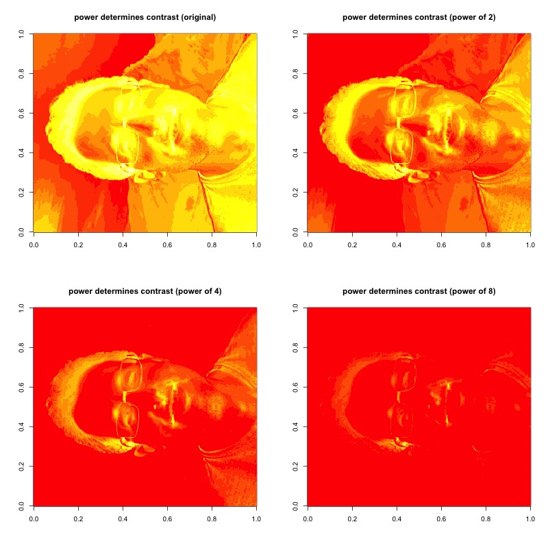
Next, we sample points proportional to the (powered) intensity level, add a bit of random noise and then plot the sample points along the x and y axis. In the picture below, you can really see how the power is very important to control the contrast levels.

Happy sampling!

	library(jpeg) # or png, depending on your image (replace readJPEG with readPNG)
	y <- readJPEG("rafa.jpeg") # You can get this off Google if you want to test it.
	jpeg("channels1to3.jpeg", width = 1200, height = 800)
	par(mfrow=c(2,3))
	image(y[,,1], main = "Channel 1")
	image(y[,,2], main = "Channel 2")
	image(y[,,3], main = "Channel 3")
	image(y[,,1], main = "Channel 1", col = rgb(seq(0, 1, by = 0.05), 0, 0))
	image(y[,,2], main = "Channel 2", col = rgb(0, seq(0, 1, by = 0.05), 0))
	image(y[,,3], main = "Channel 3", col = rgb(0, 0, seq(0, 1, by = 0.05)))
	dev.off()
	gs <- 1-(y[,,1] + y[,,2] + y[,,3])/3 # get intensity of blackness by averaging RGB channels
	# pick contrast: power determines contrast, may need tinkering depending on your initial image, skin tone, background, etc.
	jpeg("contrasts.jpeg", width = 800, height = 800)
	par(mfrow=c(2,2))
	image(gs, main = "power determines contrast (original scale)")
	image(gs^2, main = "power determines contrast (power of 2)")
	image(gs^4, main = "power determines contrast (power of 4)")
	image(gs^8, main = "power determines contrast (power of 8)")
	dev.off()
	jpeg("samplepoints.jpeg", width = 800, height = 800)
	par(mfrow=c(2,2))
	prob <- gs
	pts <- sample(length(prob), 10000, prob=prob, replace=TRUE) # sampling points proportional to the (powered) intensity
	coords <- jitter(arrayInd(pts, .dim=dim(gs))) # making coordinates with some random jitter
	plot(coords[,2], -coords[,1], pch=16, cex=0.5, main = "Points sampled on original intensity scale")
	prob <- gs^2
	pts <- sample(length(prob), 10000, prob=prob, replace=TRUE) # sampling points proportional to the (powered) intensity
	coords <- jitter(arrayInd(pts, .dim=dim(gs))) # making coordinates with some random jitter
	plot(coords[,2], -coords[,1], pch=16, cex=0.5, main = "Points samples on powered intensity scale\n(power of 2)")
	prob <- gs^4
	pts <- sample(length(prob), 10000, prob=prob, replace=TRUE) # sampling points proportional to the (powered) intensity
	coords <- jitter(arrayInd(pts, .dim=dim(gs))) # making coordinates with some random jitter
	plot(coords[,2], -coords[,1], pch=16, cex=0.5, main = "Points samples on powered intensity scale\n(power of 4)")
	prob <- gs^8
	pts <- sample(length(prob), 10000, prob=prob, replace=TRUE) # sampling points proportional to the (powered) intensity
	coords <- jitter(arrayInd(pts, .dim=dim(gs))) # making coordinates with some random jitter
	plot(coords[,2], -coords[,1], pch=16, cex=0.5, main = "Points samples on powered intensity scale\n(power of 8)")
	dev.off()
	jpeg("rafa.jpeg", width = 400, height = 450)
	par(mfrow=c(1,1))
	prob <- gs^8
	pts <- sample(length(prob), 10000, prob=prob, replace=TRUE) # sampling points proportional to the (powered) intensity
	coords <- jitter(arrayInd(pts, .dim=dim(gs))) # making coordinates with some random jitter
	plot(coords[,2], -coords[,1], pch=16, cex=0.5, ann = FALSE)
	dev.off()

view raw SamplingPointsBasedOnIntensity.r hosted with ❤ by GitHub